


Junpei Hirano
In climatology, we use values called “anomalies” to understand the average state of climatic elements (atmospheric pressure, temperature, precipitation, sunshine duration, and solar radiation, etc.). The “normal” is defined as the average value of climatic factors during the past 30 years. Since the average value changes due to climate change such as global warming, the normal is updated every ten years. For example, for the 10-year period from 2011 to 2020, the 1981-2010 average was used as the “normal,” but it was updated in 2021, and for the 10-year period from 2021 to 2030, the 1991-2020 average will be used as the “new normal.
In weather forecasting, the term “warmer (colder) than normal” is sometimes used, but in this case, “normal” refers to the “normal” value of temperature. In other words, the “normal value” of temperature is the standard for evaluating the warmth (coldness), etc. of each year. The difference between the temperature of each year and the normal is called the ” anomaly”. In the case of temperature, a positive anomaly indicates a warmer than normal year, while a negative anomaly indicates a colder than normal year. A map of temperature anomalies shows the distribution of areas with warmer-than-normal temperatures (positive anomaly areas) and areas with colder-than-normal temperatures (negative anomaly areas).
Similar to temperature, precipitation can also be plotted based on the “normal” value. However, in the case of precipitation, anomalies are generally expressed as the ratio of precipitation to the normal (ratio of normal to precipitation). For example, if you draw a precipitation anomaly map for a year with an El Niño or La Niña event, you can see areas with more or less rainfall than normal. Global precipitation anomaly maps for summer (June-August) and winter (December-February) of El Niño events are available on the Climate Atlas “World” page. However, as the basis for the anomalies, we have used the 43-year average for the period 1979-2021, for which precipitation data are available, instead of the 30-year “normal. Green-colored areas indicate areas of higher-than-normal rainfall, while brown-colored areas indicate areas of lower-than-normal rainfall. It can be seen that in El Niño years, there is more rainfall in the eastern tropical Pacific and less in the western tropical Pacific.
Furthermore, by comparing the precipitation anomaly map with the SST anomaly map, we can see the relationship between SST anomalies and precipitation anomalies. For example, in the “Winter DJF SST anomaly map for El Niño years”, the eastern tropical Pacific is colored red, indicating that SSTs are higher than normal. In an El Niño year, the sea surface temperature in this region is high, which activates cumulus convection and leads to heavy rainfall.
Global precipitation anomaly maps for summer (June – August) and winter (December – February) La Niña years show the opposite pattern (heavy rainfall in the eastern tropical Pacific and less rainfall in the western tropical Pacific). In La Niña years, sea surface temperatures (SSTs) drop below normal in the eastern tropical Pacific (see SST anomaly distribution in La Niña years), which suppresses cumulus convection and results in less rainfall.
The JCDP “Climate Atlas” will include various climate anomaly maps in the future. We recommend that you use the anomaly maps in the JCDP Climate Atlas when explaining “extreme weather” and its spatial distribution in high school geography and geology courses and in university liberal arts courses.
Hisayuki Kubota (Hokkaido University)
Meteorological observation in Japan was first started in Hakodate in 1872. The weather was also measured in Japan by using meteorological instruments before 1872, but it was conducted by individuals and the observation period was short (Zaiki et al. 2006). Therefore, we need to rely on historical diaries and documents to recover the climate during the Edo era (Yamakawa 1993).
On the other hand, the barometer was invented in the 17th century and meteorological observations were conducted in European countries. It was the age of exploration in European countries and many ships sailed to Asian countries, but Japan was a closed country during that time. Many European ships arrived near Japan in the 19th century with meteorological instruments on board. Historical ship logs are stored in libraries in each country and they attempted to rescue meteorological observation data recorded in ship logs (Brohan et al. 2006). Here we focus on Perry’s fleet who came to Japan in 1853 and 1854 in the late Edo era to open the country (Fig.1). Their ship logs are stored in the US National Archive. Here we introduce meteorological observation data recorded in their ship logs while sailing around Japan.
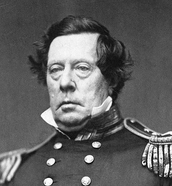
Fig.1:Matthew Perry (Wikipedia)
Figure 2 shows a ship log of USS Mississippi, one of Perry’s fleet on the 8th of July 1853 when she arrived in Tokyo Bay. Hourly meteorological observations were conducted. USS Mississippi left the east coast of the US in 1852, sailed eastward and arrived in Japan in July 1853. After that, she spent Christmas in Hong Kong and arrived in Japan again in February 1854. She then sailed eastward and reached the east coast of the US. Meteorological observation data are digitized and recovered from the records of USS Mississippi ship logs.
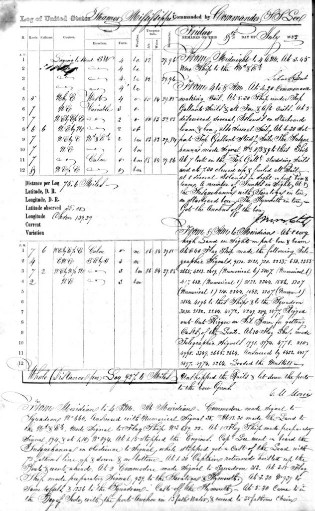
Fig. 2:Ship log of USS Mississippi on 8th July 1853 when she arrived in Tokyo Bay
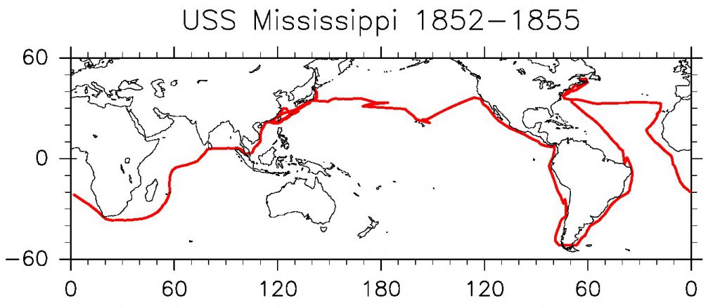
Fig. 3:Ship track of USS Mississippi during 1852-1855
Figure 4 shows the ship track USS Mississippi sailed along East Asia. Fig. 5 shows pressure, wind and existence of rain during 6-8th June when she anchored off the coast of Shimoda. Pressure dropped, associated with rain during 6-7th June, and then northerly wind intensified which indicates a low-pressure passage. Lightning stroke at Edo was recorded on 7th June 1854 in Bukou chronology (Taguchi 1943). It might be related to this low-pressure passage.
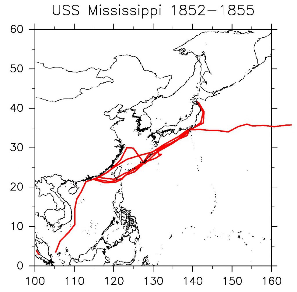
Fig.4:Ship track of USS Mississippi sailed along East Asia
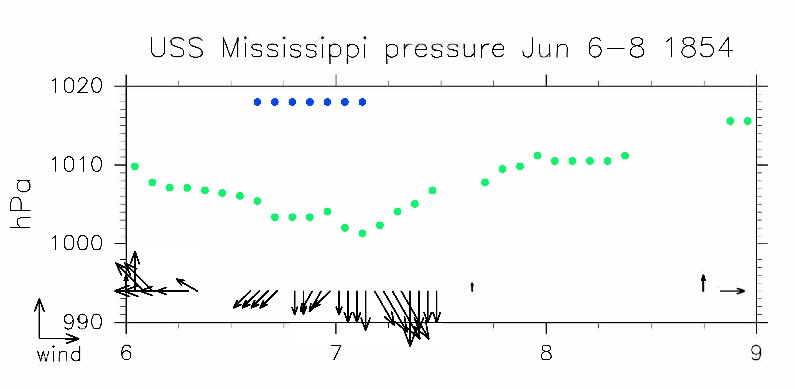
Fig.5:Pressure (green dots), wind (arrows), and existence of rain (blue dots) during 6-8 June 1854
It is known that ships of more than 10 countries sailed along East Asia during the 18th to 19th centuries. For example, more than 10,000 ship logs were found and stored in the UK library. We expect to elucidate the climate around Japan during the Edo era in the future by using meteorological observation data recorded in European and American ship logs (Kubota 2018, Kubota et al. 2018a,b).
References
Brohan, P., R. Allan, J. E. Freeman, A. M. Waple, D. Wheeler, C. Wilkinson and S. Woodruff, 2009: Marine observations of old weather, Bull. Amer. Meteor. Soc., 90, 219-230.
Kubota, H., 2018: Meteorological observation records in Hokkaido during the 18th to 19th century, “Saihyo”, 84, 3.
Kubota, H., R. Allan, C. Wilkinson, P. Brohan, K. Wood, M. Mollan, 2018a: Recovery of climate around Japan during the late Edo era using meteorological observation data recorded in foreign ship logs sailed to Japan, Meteorological Society of Japan Fall meeting 2018, B366.
Kubota, H., R. Allan, C. Wilkinson, P. Brohan, K. Wood, M. Mollan, 2018b: Recovery of Japan climate during late Edo era by foreign ship logs, The association of Japanese Geographers Spring meeting, 532.
Taguchi, T., 1943: Overview of historical weather events in Japan, Central Meteorological Observatory of Tokyo Japan, Chijin Shokan Co. Ltd.
Yamakawa, S., 1993: Natural disaster and climate change during little ice age, Chigaku Zasshi, 102, 183-195.
Zaiki, M., G. P. Konnen, T. Tsukahara, P. D. Jones, T. Mikami and K. Matsumoto, 2006: Recovery of nineteenth-century Tokyo/Osaka meteorological data in Japan, Int. J. Climatol. 26: 399–423.
Junpei Hirano
An American Christian missionary, James Curtis Hepburn(Fig1)is known for the “Hepburn’s romanization system” for transliteration of the Japanese language into Latin alphabet. He stayed in Yokohama during the 1860s as a medical missionary.
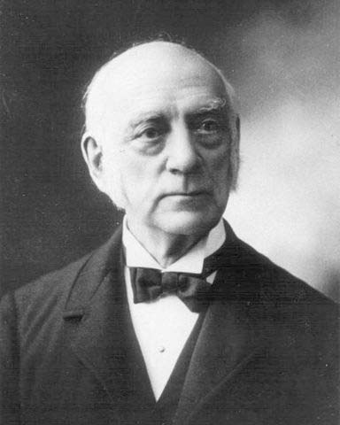
Fig1. James Curtis Hepburn https://en.wikipedia.org/wiki/James_Curtis_Hepburn
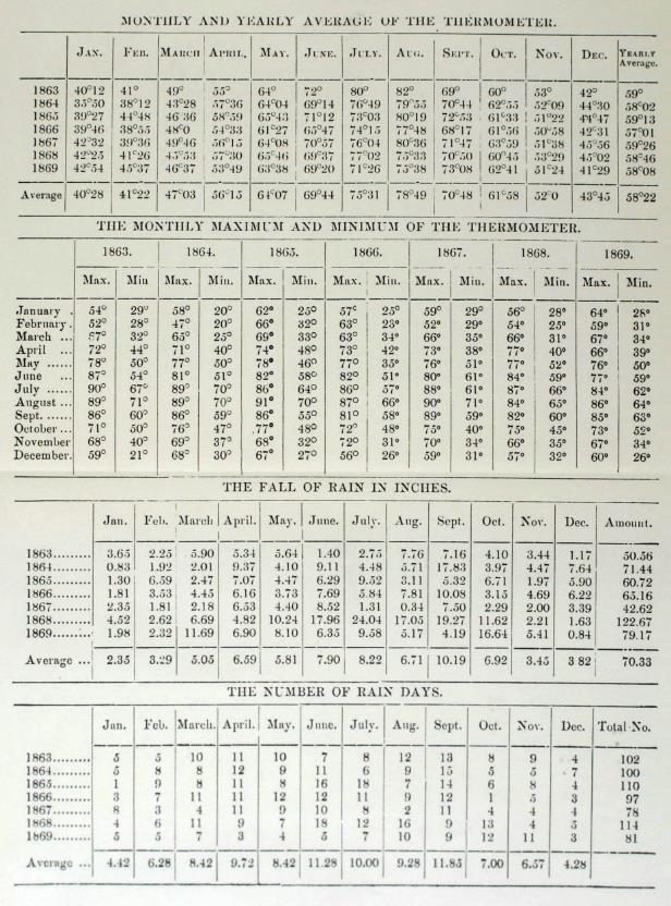
He made meteorological observations at Yokohama, from 1863 to 1869. A table of the meteorological data is presented in a bulletin of the Asiatic Society of Japan, entitled “Transactions of the Asiatic Society of Japan from 22nd October 1873 to 15th July, 1874” (Hepburn, 1874). This meteorological table contains monthly maximum, mean, and minimum temperatures, monthly precipitation, and the number of rainy days in each month (Table1). This series is archived in the Meiji Gakuin Historical Museum in Tokyo.
Table1 Meteorological table by J.C.Hepburn (Hepburn,1874)
Compared to pressure and temperature data, precipitation data in Japan are rare prior to the 1870s, when official meteorological observation by the Japan Meteorological Agency (JMA) started. Therefore, his observation is essential for analyzing precipitation variability pre-JMA period. We analyzed inter-annual variations of precipitation based on Hepburn’s observation. As a result, we detected unusually heavy rainfall during summer of 1868, whereas the summer of 1867 was characterized by extremely low precipitation (Fig2). These characteristics are in accordance with the meteorological disaster records throughout Japan in both years (Hirano et al., 2018). Therefore, these unusual climate patterns were likely related to large-scale atmospheric circulation patterns around Japan.
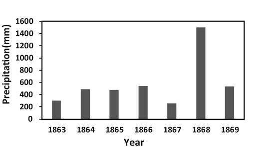
Fig2. Interannual variation of summer (JJA) precipitation at Yokohama for the period 1863-1869 (Hirano et al.,2018).
References
Hepburn, J.C. (1874): Meteorological tables. From observations made in Yokohama from 1863 to 1869 inclusive. Transactions of the Asiatic Society of Japan, from 22nd October, 1873 to 15th July, 1874, 244–248.
Hirano, J., Mikami,T., Zaiki,M. and Nishina, J.(2018):Analysis of precipitation data at Yokohama Japan, from 1863 to 1869 observed by J.C. Hepburn. Journal of Geography(Chigaku Zasshi), 127, 531-541.
Masumi Zaiki and Gunther Konnen
The observations were taken at Dejima by the Chief of the Trade Factory, J. Cock Blomhoff for 1819-1823 and then by the medical doctor P.F. von Siebold for 1825-1828 and are of air temperature, and of pressure and humidity. The data by Blomhoff are in von Siebold’s handwriting and apparently copied by him from an older document. The data by von Siebold for 23 Sept 1827-1828 are in two versions: one apparently being the originals in his own handwriting and a copy by an anonymous copyist. For the period Jan-Dec 1825, there were parallel readings in Tokyo (Figure); von Siebold also observed during his journey from Nagasaki to the Palace of the Shogun in Edo (now Tokyo) during Mar-July 1826.
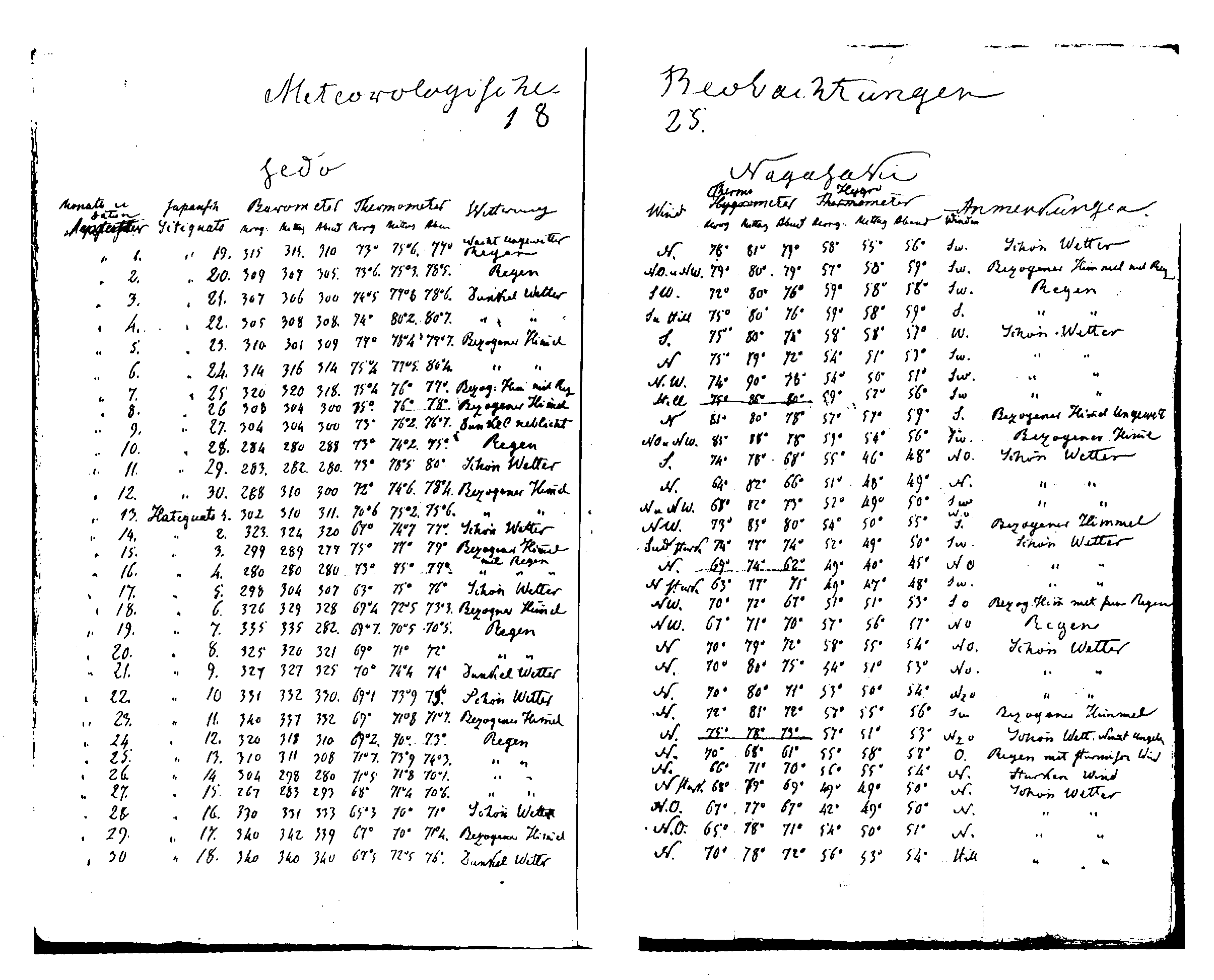
Thermometer readings were made in full degrees Fahrenheit. In the period 1819-1822, the temperature sometimes refers to readings inside the building also. Pressure is recorded only in the von Siebold period. The von Siebold pressure readings after 22 Sept 1827 were in English inches (a unit of 2.5400 cm) divided in decimals. However, the von Siebold readings Nov 1826-22 Sept 1827 are in non-English inches, which are divided in lines according to the duodecimal system (12 lines = 1 inch). From the heights of the barometer we inferred that the unit refers to French inches (a unit of 2.7070 cm).
In the 1819-1828 observations, only von Siebold recorded air humidity. It was measured by his home-made hygrometer ‘manufactured from a hair of a Japanese beauty, which was scalded in soda and then in pure water’.
The pressure and temperature observations were usually taken three times a day, referred to as ‘Morgen’, ‘Mittag’, and ‘Abend’ (morning, midday and evening). There is no explicit mention of the observation hours in the von Siebold documents. Fitting to the annual mean diurnal course of Nagasaki Observatory III 1978-1999 reveals an observation schedule 6:00, 12:00 and 22:00 Local Time (LT), where Dejima LT = UTC + 8:40.
A primary problem of the early instrumental period is the poor coverage outside Europe in the early 19th and 18th centuries. Among the many blank spots is Japan, where the official meteorological network by JMA started in the 1870s. These Blomhoff/von Siebold records extend its start back from 1878 to 1819, the significance of the data reaches further than just an extension of the Japanese instrumental record back in time. First, the recovered series happens to be in a region of the Earth that is poorly covered by instrumental data; second, it overlaps with the long daily series of visual weather reports as documented in diaries of Japanese administrators during the Edo period (1603-1868) at many places in Japan.
Takehiko Mikami
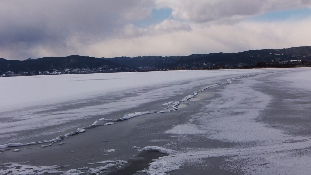
A couple of straight lines of sharp upheaval of ice, called Omiwatari on the frozen surface of Lake Suwa in central Japan, appeared for the first time in 5 years on February 2, 2018. This is a follow-up report of my column on December 27, 2017.
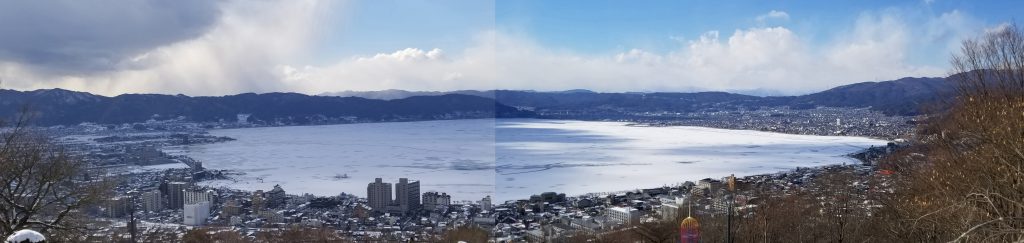
Snow-covered frozen Lake Suwa viewing from “Tateishi” Park (Photo taken by T.Mikami on 4 February, 2018)
In this winter, we have a very cold weather here in Japan, and Omiwatari phenomena occurred after almost complete freezing of the lake. Daily mean temperature at Suwa observatory in this January was -1.3 degrees, which is around same as normal means. Also the number of days with lowest temperatures below -10 degrees, which is indispensable for Omiwatari occurrence, was omly two days.
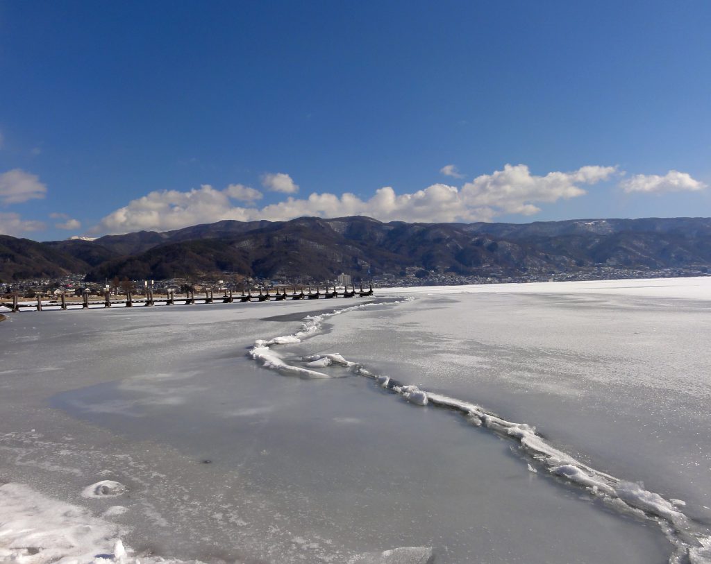
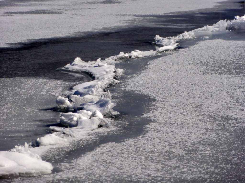
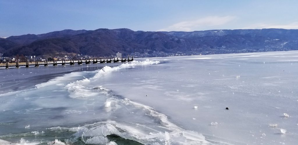
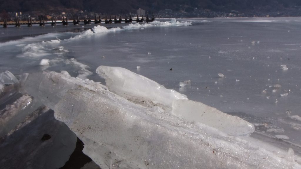
Omiwatari crossing on Lake Suwa (Photo taken at Akasunazaki by T.Mikami on 4 February, 2018)
Omiwatari crossing on Lake Suwa (Photo taken at Takagi by T.Mikami on 4 February, 2018)
According to legend, Omiwatari is said to be the footprints of God “Takeminakata-no-kami” of the Upper Suwa Shrine, who walks on the frozen lake to visit Goddess “Yasakatome-no-kami” of the Lower Shrine. The routes of Omiwatari would be different in either case due to the changes in temperature and thickness of lake ice.
Omiwatari viewing ceremony was held by “Yatsurugi” Shinto shrine priests on 5th February, and harvests and economy in this year were predicted by referring to the past documentary data for Omiwatari crossing routes.
Additional Information
The range of Omiwatari was further pushed up due to the subsequent cold weather conditions at Suwa, where daily minimum temperatures dropped down to -10.9 degrees on 8 February and -11.3 degrees on 9 February.
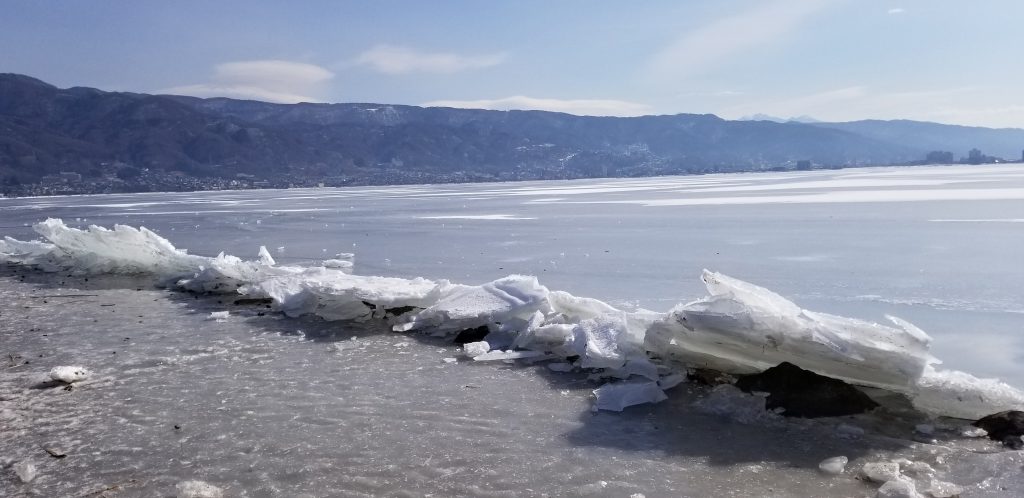
Omiwatari crossing on Lake Suwa (Photo taken at Akasunazaki by T.Mikami on 10 February, 2018)
